
Many of you reading this would have chosen to do science after learning about things like worm holes and parallel universes from popular science articles and TV shows. But how did we ever reach these ideas? Is there any actual mathematical basis behind these arguments? To answer these questions, I would try to guide you through an actual project on theoretical cosmology that I undertook last summer under a FRS string theorist (who now started working on QI but that is a different story).
Theoretical cosmology is a vast subject. The niche I worked on dealt with analysing various vacuum solutions of the Einstein equation. Lets start with a short introduction.
The Einstein equations (written below) are a set of 10 partial differential equations. The summation convention (also devised by Einstein and, to quote T Padmanabhan, sometimes called his 2nd biggest contribution to physics; the 1st being GR of course) makes it possible to write everything in the compact form you see below.
Rμν is called the Ricci curvature tensor, and its an object purely from Riemmanian geometry. Tμν is the stress energy tensor which has nothing to do with geometry and rather comes from the physical properties of the object we are looking at. The equation relating these two was Einstein's genius.
The solutions to these equations are various metrics in space time. A metric, in simple words, is just the distance between two points in four dimensional (3+1) space time. The simplest metric is a trivial solution of the Einstein equation known as the Minkowski metric and is shown below. Rμν for the Minkowski metric is zero everywhere, which just means that the space time described is flat everywhere.

A little more complex is the Schwarzschild metric, first derived by Karl Schwarzschild months after Einstein published his general theory of relativity in 1915. This metric describes the simplest black hole, as we will briefly see. The metric is shown below, in spherical coordinates.

Roger Penrose in 1950s used some fairly simple diagrams, which he called conformal diagrams, to exhibit the properties of various space time. The derivation of these diagrams are beyond the scope of this article, however, we will try to see what they represent for some interesting solutions. We will refer to them as Penrose-Carter diagrams after the authors of the first paper that was published with them.
The project in its entirety was about deriving a Penrose-Carter diagram to probe the properties of a Kerr-Newman metric, which is a simply a charged and rotating black hole. Surprisingly, one does not need to know a lot of general relativity to take on a project like where we are only interested in the solutions which GR presents us and not with the how and why of getting to those solutions.
Before starting this project, I was expected to be well versed in special relativity, and just a little bit of differential geometry. After that, I worked on simple examples, deriving Penrose-Carter diagrams and analysing the results. How exactly? Well, lets take a look at the diagram for a simple Schwarzschild black hole. An important fact to note here is that we suppress the angular dimensions (θ, φ) for simplicity. Our diagrams can thus be now two dimensional. This move will not harm us in any way, because we are only going to look at spherically symmetric metrics.
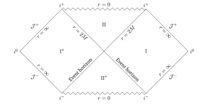
Now, lets see what this is all about. The r=0 swiggly lines denote the singularity. We wont talk about what happens there because that is physics heresy.
Next we have the r=2M lines dividing the region diagram into 4 regions. These lines denote the event horizons; if you cross this, its goodbye. Finally, we are bounded by r=∞. Our diagrams thus covers the entire domain of r ∈ (0,∞).
In a Penrose-Carter diagram, light rays are always at an angle π/4 with the horizontal and they can only travel up. If we look at regions I and II, light rays emanating from r=∞ falls into the black hole at r=0. No surprises there.
Now consider regions I* and II*. If we follow the rules, it seems light rays emanate from the singularity and fall race towards r=∞. But then surely, the singularity at r=0 in region II* cannot describe a black hole. For starters, it emits light, it wont even be black!
Indeed, the singularity in question does not belong to a conventional black hole. It is sometimes called a white hole; a white hole would not pull mass towards it but push it away. Unfortunately, we haven't yet detected such a fascinating object. But a question you can ask here is are the regions I and I* the same? And if you did I would say congratulations for reading my mind but the answer is not at all. If you look at the diagram long enough, you can convince yourself that any ray of light from region I can never make it to region I* and vice versa. And if light can't, nothing else can. This can be seen in the diagram too. Any other object's trajectory (sometimes called a geodesic or a world line; light rays are called null geodesics) will have an angle greater that π/4, as it must travel with a speed less than c which makes it clear that its not crossing into the other region by any means. Therefore these regions should represent entirely different universes, as they are causally disconnected.
After this, came a few other metrics which were not as simple. The Kerr-Newman metric was the most complicated, and it was proving very difficult to simplify. When I had 7 - 10 days left in my internship, I stumbled upon a devilishly simple fact. It turned out that the causal structure of the Kerr solution (which I had already solved), was entirely similar to that of the Kerr-Newman solution. I was able to prove this fact, and I finished my internship early.
Looking at the Kerr-Newman metric is out of the scope of this discussion. We will however, look at another very intresting diagram. Its a particular case of the Reissner-Nortstorm solution, which is a static black hole carrying a non zero electric charge.
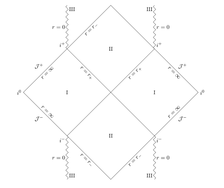
This diagram extends to infinity in the vertical direction with the same pattern repeated. Before diving into the diagram, lets take a look at the metric.

Here, e represents the total charge carried by the black hole; $e=0$ reduces exactly to the Schwarzschild solution.
The terms for the charge, however, completely changes the causality of our black hole. Lets start with the boundary labeled J- A light ray again moving at $\pi/4$ to the horizontal, hits the boundaries r=r+ and r=r- before finally hitting the singularity at region III. These boundaries represent event horizons; the point of no return. Thus this particular black holes has two event horizons guarding the singularity.
So what does this all mean? Well, region I is the part of the universe outside the black hole. Region II is an intermediate region. If you fall into II you there is no way you can avoid III. But there is a catch. Notice how I did not said that you are doomed if you fall into II; its because you are not.
Well how is that possible? The singularity of a charged black hole is vertical (or timelike). This implies any object other than light, can avoid the singularity. But how? Remind yourself that non null geodesics' angle with the horizontal must belong to π/4, π/2. With this fact in mind, its easy to see that your average astronaut going into the black hole can avoid the singularity entirely. However, he cannot come back to his own universe, which is forever in his past.
But if not the singularity or back to his universe then where? This is where it gets interesting. As we already said, the diagram is infinite. So then we can imagine our astronaut going through the top of the diagram and appearing at the bottom in the same region III. Now he can cross the event horizons to arrive at region I. But this new region I is not his own universe; which was, if you recall, forever in his past. He can explore this place as much as he wants, but if he decides to enter a Reissner-Nortstorm black hole, he would need to say goodbye to this new universe too and find a new home.
This suggests there exists infinite universes complete with portals to travel through them. And I would say that the GR does not in fact deny it. But a physical theory is a mathematical construct. A real black hole has irregularities and the Penrose-Carter diagrams we have drawn here do not exactly do justice to them. [These irregularities actually arise because the way a black hole forms. See reference 1 for more details on this]. Without delving into details, I would just hint at the fact that for all we know, all these fantastical revelations might be nothing more than the t < 0 solutions you get when solving simple kinematics i.e, unphysical.
But if we stopped to study things that might not exist then a lot of physicists are losing their jobs (A certain field comes to mind; something to do with no experimental proof for 40 years now). However, theories are to theorists what music is to musicians; to have fun, you must do it for yourself and not for the audience.
Finally, to wrap things up, we learnt that general relativity does predict some very interesting phenomena. And I would agree that these are indeed exciting. However, science fiction has paid way to much attention to these ideas. So much so that for many people, that is what physics stands for! Of course, as you just read, there is a lot to physics than that. Reaching these results took around 50 years, and along the way we learnt a lot more about GR and the universe. Unfortunately, we also learnt that GR does not work every where and the some physicists actually believe that is it a special case of a more general theory. Surely, theoretical cosmology is far from other. A lot of adventures lie ahead. Who knows, maybe some of you reading this become part of it!
I would like to end with a quote by the hero of this article.
It is always the case, with mathematics, that a little direct experience of thinking over things on your own can provide a much deeper understanding than merely reading about them.
-Roger Penrose
References
- Hawking, S. W.; Ellis, G. F. R. , The large scale structure of space-time. Cambridge University Press, Oxford, UK, 1973
- Boyer, R. H.; Lindquist, R. W. (1967), `Maximal analytic extension of the Kerr metric', J. Math. Phys. 8, 265-81
- Kruskal, M. D. (1960), `Maximal extension of Schwarzschild metric', Phys. Rev., 119, 1743-5
- Ferrari, V.; Gualtieri L. (2011), `Black holes on general relativity', Dipartimento di Fisica, Universita degli studi di Roma “Sapienza''
- http://www.roma1.infn.it/teongrav/leonardo/bh/bhcap12.pdf

.svg)
.png)